‘Over-plotting’
Many times we want strike-zone plots of many pitches at once (for example, see Jim’s great post on visualizing Cliff Lee’s pitches). When dealing with many pitches, it’s easy to plot points on top of one another, which can lead to a mis-representation of the true density of pitches. In the data visualization community, this problem is generally known as “over-plotting”. Stephen Few has a great overview of things you can do to avoid over-plotting. I will apply a couple of these techniques to help visualize every pitch thrown by Clayton Kershaw’s during 2013 season.
Data collection
Before we start making plots, let’s grab the necessary data using techniques discussed in my last post.
library(dplyr)
setwd("~/pitchfx") # My directory that contains a SQLITE DB with PITCHf/x
db <- src_sqlite("pitchRx.sqlite3")
atbats <- tbl(db, "atbat") %>%
  filter(date >= '2013_01_01' & date <= '2014_01_01') %>%
  filter(pitcher_name == 'Clayton Kershaw')
pitches <- tbl(db, "pitch")
kershaw <- collect(inner_join(pitches, atbats, by = c("num", "gameday_link")))
Just to feel for the size of this data, let’s count the number of different pitch types thrown by Kershaw broken down by batter stance:
kershaw %>%
  group_by(pitch_type, stand) %>%
  summarise(count = n()) %>%
  arrange(desc(count))
## Source: local data frame [11 x 3]
## Groups: pitch_type
##
## pitch_type stand count
## 1 FF R 1831
## 2 SL R 770
## 3 FF L 594
## 4 CU R 405
## 5 SL L 211
## 6 NA R 109
## 7 CH R 98
## 8 CU L 97
## 9 NA L 22
## 10 IN R 7
## 11 CH L 2The pitch type abbreviations ‘FF’, ‘SL’, ‘CU’, ‘CH’, and ‘IN’ stand for (respectively) ‘four-seam fastball’, ‘slider’, ‘curveball’, ‘change-up’, and ‘intentional walk’. The intentional walks won’t be very interesting from a visual standpoint, so let’s get rid of them:
kershaw <- filter(kershaw, pitch_type != "IN")Strike-zones made easy with strikeFX
The strikeFX function from the pitchRx package was created to provide a quick yet flexible way to visualize PITCHf/x data. Even if you’re not versed in ggplot2, it’s easy to make strike-zone plots:
library(pitchRx)
strikeFX(kershaw)
# strikeFX knows to use the 'px' and 'pz' columns for 'x' and 'y'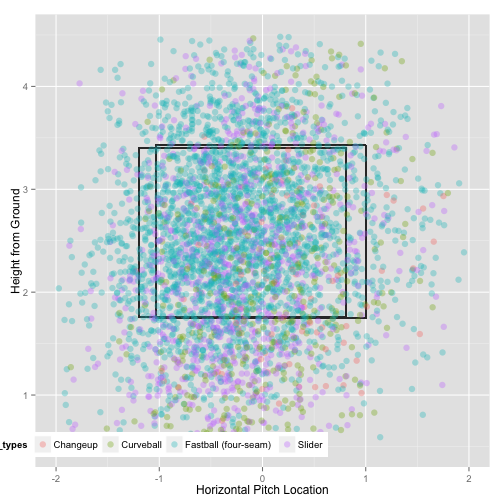
The two black rectangles correspond to left-handed and right-handed strike-zones created using the approach Mike Fast suggests in this post. Since the strike-zone depends on the batters height, strikeFX has an option to adjust the vertical pitch locations to account for the “averaged” strike-zones on the plot. strikeFX also uses a variety of defaults (such as coloring points by the pitch type) that can be altered. In addition to altering defaults, arguments to strikeFX can also add elements such as contour lines to the graphic (see the documentation for other arguments). Note that the type variable contains abbreviations ‘B’, ‘S’, and ‘X’ which stands for (respectively) ‘Ball’, ‘Strike’, and ‘Hit in play’.
strikeFX(kershaw, color = "type", point.alpha = 0.5, adjust = TRUE, contour = TRUE)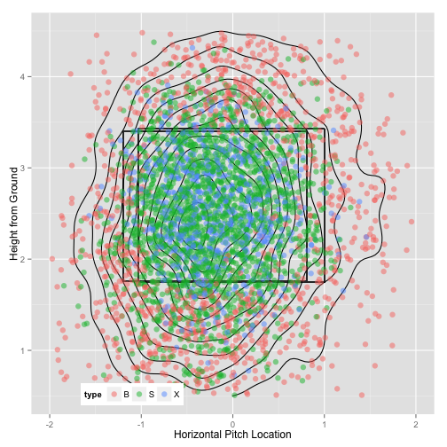
If you’re familiar with ggplot2, we can take advantage of it’s arithmetic approach to modify graphical elements, add complexities, and customize the appearance. To demonstrate, I’ll take essentially the same plot, but place pitches thrown to left-handed and right-handed batters into separate plots (with facet_grid), move the location of the legend (with theme), fix the ratio between the axes and the plot presentation (with coord_equal), and change the background from gray to white (with theme_bw).
strikeFX(kershaw, color = "type", point.alpha = 0.2,
         adjust = TRUE, contour = TRUE) + facet_grid(. ~ stand) +
  theme(legend.position = "right", legend.direction = "vertical") +
  coord_equal() + theme_bw()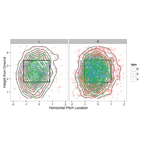
Now it’s clear that the density estimate (that is, the contour lines) in the second plot was heavily influenced by pitches thrown to right-handed batters. We can gain further insight by simply adding pitch_type to facet_grid.
strikeFX(kershaw, color = "type", point.alpha = 0.1,
         adjust = TRUE, contour = TRUE) + facet_grid(pitch_type ~ stand) +
  theme(legend.position = "right", legend.direction = "vertical") +
  coord_equal() + theme_bw()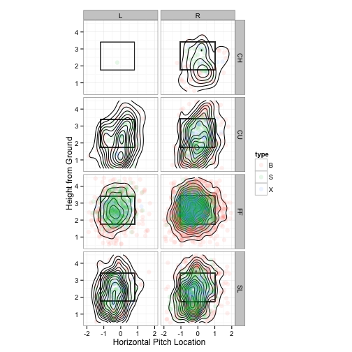
Now it’s clear that a much lower proportion of strikes occur outside of the strike-zone for four-seamers (compared to the other pitch types). Also, the location of highest density is much higher in the strike-zone for four-seamers (compared to the other pitch types). This shouldn’t be that surprising, but reassuring that the data matches our intuition.
In addition to using a categorical variable for color assignment, we can also use a numerical variable and strikeFX will automatically know to use a one-way color scale:
strikeFX(kershaw, color = "end_speed", point.alpha = 0.1,
         adjust = TRUE, contour = TRUE) + facet_grid(pitch_type ~ stand) +
  theme(legend.position = "right", legend.direction = "vertical") +
  coord_equal() + theme_bw()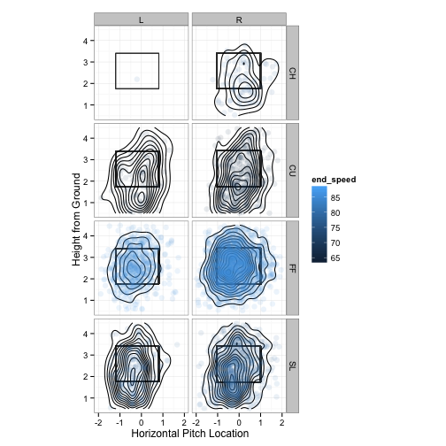
From this plot, it’s fairly obvious that end_speed is a good indicator of pitch_type, except that it doesn’t provide a great distinction between change-ups (CH) and sliders (SL). There are a number of other varibles that should be a decent predictor of the pitch type, including spin direction. If we wish to use spin direction instead of speed as a coloring variable, it’s not a great idea to use the same one-way color scale since spin direction is measured as an (0 to 360 degree) angle. In other words, a different scale is needed since a spin direction of 0 is closer a spin direction of 360 (compared to, say, 180).
It is recommended that one-way color scales use constant hue, but vary chroma and luminance. That explains why the points in the previous plot vary between dark blue and light blue. With respect to spin direction, we definitely want to vary hue, but probably want to hold chroma and luminance constant (thanks Thomas Lumley). Upon researching this idea, I discovered that the I’ve heard rumors are true…colorimetry is hard/complicated. Thankfully, ggplot2 has a simple built-in solution to our issue – scale_colour_gradientn. This provides a way to use “smooth transitions” between an arbitrary number of colors. Although this approach allows chroma and luminance to vary, I think the result is reasonable:
strikeFX(kershaw, color = "spin_dir", point.alpha = 0.3,
         adjust = TRUE, contour = TRUE) + facet_grid(pitch_type ~ stand) +
  theme(legend.position = "right", legend.direction = "vertical") +
  coord_equal() + theme_bw() + scale_colour_gradientn(colours = rainbow(7))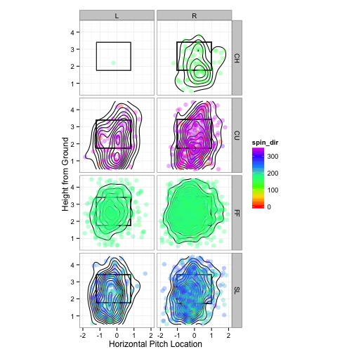
A few things I take away from this plot is that spin direction:
- provides a nice distinction between curveballs and fastballs.
- provides a decent distinction between sliders and changeups.
- is more variable amongst sliders than any other pitch type.
- for sliders is somewhere between curveballs and fastballs on average.
- for changeups is slightly lower on average compared to fastballs.
For more demonstrations of the capabilities of strikeFX, check out the pitchRx introduction page and the RJournal article.