MLBAM’s website hosts a wealth of data that informs the MLB Gameday application. Most notably, this website hosts pitch-by-pitch (ie, PITCHf/x) and play-by-play data. pitchRx provides a simple interface to acquire a good portion of Gameday data (see Table 1 of my paper), but there is a significant amount that isn’t directly accessible using pitchRx::scrape. This post will show you some general techniques to acquire and manipulate data from this website.
Constructing Gameday urls
When scraping data off the web, typically the first task is to construct urls that point to the information of interest. Sometimes this is difficult, but thankfully, the Gameday site structure urls in a sensible fashion. In fact, if we are searching for game specific data, the full address can be constructed from the Gameday identifier. To demonstrate, let’s grab Gameday identifiers for MLB and Triple-A games played in August of 2014 (this post has more on searching Gameday identifiers with regular expressions).
library(pitchRx)
# Load gameday identifiers
data(gids, package = "pitchRx")
data(nonMLBgids, package = "pitchRx")
# Subset MLB identifiers to August, 2014
MLBids <- gids[grepl("2014_08_[0-9]{2}", gids)]
# Subset to Triple-A games in August, 2014
AAAids <- nonMLBgids[grepl("2014_08_[0-9]{2}_[a-z]{3}aaa_[a-z]{3}aaa", nonMLBgids)]
ids <- c(MLBids, AAAids)
ids[1]
## [1] "gid_2014_08_01_phimlb_wasmlb_1"The function pitchRx::makeUrls can then be used to pre-append the path required to reach ‘game directories’.
paths <- makeUrls(gids = ids)
paths[1]
## [1] "http://gd2.mlb.com/components/game/mlb/year_2014/month_08/day_01/gid_2014_08_01_phimlb_wasmlb_1"Within each game directory, there are a bunch of files (to see them, click on the link above). Note that pitchRx::scrape has support for acquiring: miniscoreboard.xml, players.xml, inning/inning_all.xml, and inning/inning_hit.xml files; but any of these XML files can be harvested using XML2R.
Motivating XML2R
While developing pitchRx, I found myself writing a lot of redundant R code that repeatedly transformed similarly structured XML documents into a list of data frames. Through this discovery, I found a reasonable way to abstract the common tasks into a small number of functions/conventions which are bundled into a separate R package named XML2R. In fact, I have a vignette which explains how pitchRx uses XML2R to acquire PITCHf/x data. I intend to write more sports data scrapers on top of XML2R (e.g., bbscrapeR) and possibly combine them into a central R package.
From urls to observations
The fundamental idea behind XML2R is that any XML structure can be coerced into a list of observations. Here I will transform a bunch of rawboxscore.xml files into a list of observations using XML2Obs:
library(XML2R)
urls <- paste0(paths, "/rawboxscore.xml")
obs <- XML2Obs(urls) # this will take a minute
The names of this list keeps track of the XML hierarchy. In some sense, this hierarchy can be thought as defining an observational unit. XML2R has functionality for combining and creating links between observations, but we won’t cover that here. Instead, let’s take a peek at the top 5 observational units in terms of the count of observations within each level.
nms <- names(obs)
top <- sort(table(nms), decreasing = TRUE)
head(top)
## nms
## boxscore//team//batting//batter
## 26205
## boxscore//team//pitching//pitcher//strikeout
## 14047
## boxscore//linescore//inning_line_score
## 8652
## boxscore//team//pitching//pitcher
## 7153
## boxscore//team//pitching//pitcher//walk
## 5799
## boxscore//umpires//umpire
## 3349Just because, here are two observations from the most popular observational unit:
batter <- obs[grepl("^boxscore//team//batting//batter$", nms)][1:2]
batter
## $`boxscore//team//batting//batter`
## hr sac name_display_first_last pos rbi id lob bis_avg
## [1,] "0" "0" "Ryan Howard" "1B" "0" "429667" "0" ".220"
## name bb bis_s_hr bam_s_so fldg bam_s_bb hbp d e so a
## [1,] "Howard" "0" "16" "124" "1.000" "45" "0" "0" "0" "0" "1"
## bis_s_t bam_s_t sf bam_s_r bam_s_hr h bat_order bis_s_r bis_s_rbi
## [1,] "1" "1" "0" "48" "16" "0" "400" "48" "63"
## t bis_s_so bis_s_h bam_s_h ao bam_s_rbi r bam_s_e sb bis_s_d
## [1,] "0" "124" "87" "87" "1" "63" "0" "7" "0" "11"
## bam_s_d bis_s_e po ab bis_s_bb bam_avg go
## [1,] "11" "7" "12" "4" "45" ".220" "3"
## url
## [1,] "http://gd2.mlb.com/components/game/mlb/year_2014/month_08/day_01/gid_2014_08_01_phimlb_wasmlb_1/rawboxscore.xml"
##
## $`boxscore//team//batting//batter`
## hr sac name_display_first_last first_sac pos id rbi lob
## [1,] "0" "1" "Roberto Hernandez" "262" "P" "433584" "0" "2"
## bis_avg name bb bis_s_hr bam_s_so fldg
## [1,] ".056" "Hernandez, R" "0" "0" "17" "1.000"
## first_two_out_risp_lob bam_s_bb hbp d e so a sf bam_s_r
## [1,] "95" "0" "0" "0" "0" "0" "0" "0" "0"
## bam_s_hr two_out_risp_lob h bat_order bis_s_r bis_s_rbi t
## [1,] "0" "1" "0" "900" "0" "1" "0"
## bis_s_so bis_s_h bam_s_h ao bam_s_rbi r sb po ab bis_s_bb go
## [1,] "17" "2" "2" "0" "1" "0" "0" "2" "2" "0" "3"
## bam_avg
## [1,] ".056"
## url
## [1,] "http://gd2.mlb.com/components/game/mlb/year_2014/month_08/day_01/gid_2014_08_01_phimlb_wasmlb_1/rawboxscore.xml"
Note that each observation (or each list element) is a character matrix with one row. This makes it easy to row bind observations at a later point.
str(batter)## List of 2
## $ boxscore//team//batting//batter: chr [1, 1:46] "0" "0" "Ryan Howard" "1B" ...
## ..- attr(*, "dimnames")=List of 2
## .. ..$ : NULL
## .. ..$ : chr [1:46] "hr" "sac" "name_display_first_last" "pos" ...
## $ boxscore//team//batting//batter: chr [1, 1:43] "0" "1" "Roberto Hernandez" "262" ...
## ..- attr(*, "dimnames")=List of 2
## .. ..$ : NULL
## .. ..$ : chr [1:43] "hr" "sac" "name_display_first_last" "first_sac" ...From observations to data frame(s)
For our purposes, I just want to see how audience attendance differs across ballparks in both the MLB and Triple-A. To investigate, I’ll just grab the “boxscore” observational unit:
bs <- obs[grepl("^boxscore$", nms)]
bs[1]
## $boxscore
## wind game_type venue_name home_sport_code
## [1,] "15 mph, L to R" "R" "Nationals Park" "mlb"
## attendance official_scorer game_pk date status_ind
## [1,] "28,410" "Dave Matheson" "382175" "August 1, 2014" "F"
## home_league_id elapsed_time game_id venue_id
## [1,] "104" "2:28" "2014/08/01/phimlb-wasmlb-1" "3309"
## weather gameday_sw
## [1,] "79 degrees, cloudy" "P"
## url
## [1,] "http://gd2.mlb.com/components/game/mlb/year_2014/month_08/day_01/gid_2014_08_01_phimlb_wasmlb_1/rawboxscore.xml"Now, since scores is a list of observations all with the same observational unit, we can collapse the observations into a matrix.
unique(names(bs))
bs.mat <- collapse_obs(bs)
bs.mat[1:5, !grepl("url", colnames(bs.mat))] #first 5 records without "url" column
## wind game_type venue_name
## [1,] "15 mph, L to R" "R" "Nationals Park"
## [2,] "3 mph, L to R" "R" "Oriole Park at Camden Yards"
## [3,] "7 mph, In from CF" "R" "Progressive Field"
## [4,] "8 mph, In from CF" "R" "Comerica Park"
## [5,] "0 mph, None" "R" "Marlins Park"
## home_sport_code attendance official_scorer game_pk date
## [1,] "mlb" "28,410" "Dave Matheson" "382175" "August 1, 2014"
## [2,] "mlb" "39,487" "Jim Henneman" "382177" "August 1, 2014"
## [3,] "mlb" "27,009" "Bob Maver" "382179" "August 1, 2014"
## [4,] "mlb" "39,052" "Dan Marowski" "382170" "August 1, 2014"
## [5,] "mlb" "20,410" "Ronald Jernick" "382169" "August 1, 2014"
## status_ind home_league_id elapsed_time game_id
## [1,] "F" "104" "2:28" "2014/08/01/phimlb-wasmlb-1"
## [2,] "F" "103" "2:29" "2014/08/01/seamlb-balmlb-1"
## [3,] "F" "103" "3:23" "2014/08/01/texmlb-clemlb-1"
## [4,] "F" "103" "2:56" "2014/08/01/colmlb-detmlb-1"
## [5,] "F" "104" "2:58" "2014/08/01/cinmlb-miamlb-1"
## venue_id weather gameday_sw
## [1,] "3309" "79 degrees, cloudy" "P"
## [2,] "2" "78 degrees, cloudy" "P"
## [3,] "5" "76 degrees, clear" "P"
## [4,] "2394" "81 degrees, clear" "P"
## [5,] "4169" "75 degrees, roof closed" "P"In R, matrices have homogeneous column types and XML2R will always return a character matrix. For this reason, some data cleaning is usually required. In this case, we coerce attendance to an integer type and collect a subset of the columns into a data frame (which can handle heterogeneous column types).
attendance <- as.integer(gsub("\\,", "", boxscore[,"attendance"]))
venue <- boxscore[,"venue_name"]
# this is here to tell ggplot to sort venues by their median attendance
parks <- names(sort(tapply(attendance, INDEX = venue, median)))
df <- data.frame(attendance, venue = factor(venue, levels = parks),
                 league = boxscore[,"home_sport_code"])
From data frame(s) to insight
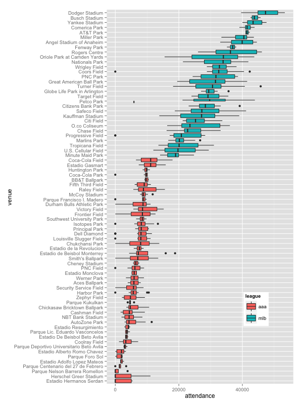
Lastly, let’s visualize the distribution of single game attendance across ballparks. Not a whole lot of surprise here, but I think it is interesting that the variance is MUCH higher in the major leagues (except for the few teams with a very loyal following – I’m looking at you Red Sox & Giants fans).
library(ggplot2)
qplot(data = df, x = venue, y = attendance, geom = "boxplot",
      fill = league) + coord_flip() +
      theme(legend.position = c(0.8,0.2))