If you haven’t read them already, go check out Brian’s great posts on pitch classification and cluster analysis. I particularly like his argument that our goal should be to “Identify all the pitches that can reasonably be classified as ‘different’ from one another”. Grouping observations into similar sets is a very common task in unsupervised settings where a response variable of interest is either unknown or doesn’t exist. There are a mind-boggling number of different methods for “learning” the “best” grouping and Brian has gracefully covered two of them (k-means and model based clustering). Here I’ll present yet another approach that relies on human perception and our ability to recognize patterns.
In Brian’s post on model based clustering, he visually inspected the fit of the model in the data space with mclust::coordProj(). This approach is limited in the sense that we can only verify how the model fits onto a scatterplot(s) between two numeric variables, but the whole data space is a higher dimensional beast. Although we are visually limited to 3 dimensions, we can still dynamically explore projections of data in high dimensions in such a way that allows us to construct a mental model of the entire space (commonly referred to as touring multidimensional data).
There are many ways to tour multidimensional data. The most common are the grand tour and the guided tour. The grand tour interpolates through random projections of the data whereas the guided tour progresses through “interesting” projections. In this post, I’ll keep things simple, and we’ll take a grand tour of Mariano Rivera’s pitches from 2011.
data(pitches, package = "pitchRx")
rivera <- subset(pitches, pitcher_name == "Mariano Rivera")
When I say a grand tour walks through random projections, I really mean that it goes through random linear combinations of all the variables that we give it (subject to some constraints). This is important since this implies that we can’t include categorical variables in the tour. Let’s use the same numeric variables that Brian did when examining Mark Buerhle’s pitches:
vars <- c("start_speed", "break_y", "break_angle", "break_length")
rivera_num <- rivera[names(rivera) %in% vars]
# ensure these variables are numeric
rivera_num[] <- lapply(rivera_num, as.numeric)
With the tourr package, it’s really easy to perform the grand tour (although, I’ve had problems running this code inside of RStudio, so you may want to run this outside of RStudio):
library(tourr)
animate(rivera_num, grand_tour(), display_xy())
We can actually mimic this functionality and make the results easier to share using animint. In fact, I’ve provided a convenience function for creating tours of PITCHf/x data called pitch_tour(). By default, pitch_tour() will use MLBAM’s pitch type classification for the point color.
devtools::source_gist("4673815529b7a1e6c1aa")
pitch_tour(rivera)
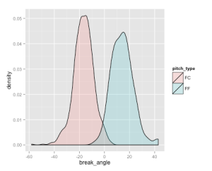
If you view the result here (best viewed with Chrome), you’ll notice that the projection begins with break_y on the y-axis and start_speed on the x-axis. There appears to be 4-5 very distinct groups/clusters of pitches along the break_y axis (I’ll return to this shortly). As the tour progresses through the random projections, you should also notice that MLBAM’s classification is almost entirely determined by the break_angle (that is, we could draw a line orthogonal to the break_angle axis that separates red points from blue points):
library(ggplot2)
rivera$break_angle <- as.numeric(rivera$break_angle)
ggplot(rivera, aes(x = break_angle, fill = pitch_type)) +
  geom_density(alpha = 0.2)
rivera$mlbam_type <- cut(rivera$break_angle, c(-100, 0, 100))
with(rivera, table(mlbam_type, pitch_type)) pitch_type
mlbam_type FC FF
(-100,0] 775 4
(0,100] 14 119However, given what we’ve seen in the tour, splitting on break_y is clearly better if our goal is to produce the most “distinct” grouping (that is, most separated from one another in the data space). In fact, a model based clustering mostly agrees with our visual intuition:
m <- mclust::Mclust(rivera_num)
rivera_num$classification <- m$classification
pitch_tour(rivera_num, color_by = "classification", out_dir = "rivera-mbc")
Of course, Rivera doesn’t have anywhere near 8 different pitch types. The point here is that the cluster analysis is fooled by the “discreteness” of break_y. Rivera’s break_y only varies from 23.6 to 24.0 and the precision of break_y measurements only goes to the tenth place. Whenever the ratio of precision to range for a numerical variable is this large, it is bound to cause problems, so we should to remove it from consideration for Rivera. Interestingly, Mark Buerhle’s break_y data is similar to Rivera’s, but the model based clustering approach doesn’t get fooled as badly. I suppose that is due to that fact that Mark has a higher number of actual types are more spread out in the data space.
mark <- read.csv("http://www.brianmmills.com/uploads/2/3/9/3/23936510/markb2013.csv")
table(mark$break_y)
23.6 23.7 23.8 23.9 24
24 521 2128 668 27 mark_num <- mark[names(mark) %in% vars]
mark_num[] <- lapply(mark_num, as.numeric)
m2 <- mclust::Mclust(mark_num)
mark_num$classification <- m2$classification
pitch_tour(mark_num, color_by = "classification", out_dir = "mark-mbc")